The goal of this assignment is to learn how to evaluate performance of your parallel program and improvements you make to it. First, you will evaluate the master-slave program you wrote for the 2nd assignment according to several metrics. Then you will try one or more modifications to its basic work queue algorithm to see whether that brings any improvement. Note that this assignment will require running more experiments as well as a good analytical write-up, but hopefully will involve less coding than the previous one. You can do this assignment either individually or with a partner. The only thing we ask is for undergraduates to pair up only with undergraduates and graduates to pair up only with graduates since you must run on different platforms.
The assignment consists of several parts. Although they each contribute a fixed portion to the overall score, it will be difficult to do well on later parts without doing well on earlier parts.
In the second assignment you had to time the overall execution your program, as well as the overhead time and the computation time for each processor. All you have to do now is run the program with different number of workers (do runs with 1, 2, 4, and 8 workers) and for each of those, run it with chunks of different size (do chunks of size 4x4, 16x16, 64x64, 256x256, and 512x512) and record the time values.
Actually, instead of the overhead and computation time for each processor, we will only use the averages of those values. So you can either modify your program to compute and output the averages by itself, or you can have have a script compute the averages after the program is finished. In the former case, which I highly recommend, you'll just need to have the workers also send back their timing values along with the output data and have the master compute the averages after all workers are done.
A few words about timing. Try not to include file I/O on the master in the measurement of total execution time. In other words, start the timer after you read the input file into memory and stop it before you write out the result. Although an important issue to consider in practice, file I/O will only make your results more difficult to interpret. Also, make sure you measure the overhead time correctly -- remember that it includes both communication and waiting.
Here are some suggestions on how to stage your long-running experiments:
Now that you have all this data, the best way to see how well you program runs under those different conditions is to generate some plots. You are welcome to plot the data in any way you want or even plot some other measurements that you find useful, but you will have to turn in the following six 2D plots in order to get full credit:
As you can see, the first graph will have four curves, graphs two through five will have three curves each and the last one will have five curves. Use logarithmic scale along the X axis for all of them (since both chunk size and number of processors grow exponentially).
There are many software packages out there that will allow you to generate these simple plots. You can use Excel or some other spreadsheet under Windows or Mac, or you can use gnuplot installed in both uAPE and APE labs. The graduate APE lab also has a program called xvgr, but its GUI is so unintuitive that you might be better off staying with command-line-oriented gnuplot. Since it really helps to be able to plot the results right after executing a particular run, I highly recommend learning some Unix plotting tool like gnuplot. Later this week we hope to add a page about using gnuplot for the plots in this assignment.
Now that you can see how the program performs under different situations, the question that comes to mind is "Can we end this assignment right here and go home?" Seriously, though. One usually would like to keep the amount of overhead in the parallel program to a minimum. Most likely, your graphs will show that while there is not that much overhead when only few large chunks are sent out, there is quite a bit of overhead when many tiny chunks are used. Try to see if you can reduce this overhead and thus improve the overall performance using one (or more) of these optimizations:
Under the most straightforward work queue implementation, as soon as the worker finishes, it sends its output to the manager, waits for another chunk to arrive and then starts another computation. While the data is being copied in and out of the buffer and while it is being transferred over the network, the worker could potentially be doing something useful. If we somehow try to arrange our communication so that by the time the worker is done with one chunk there is another one for it to compute on, then we might be able to decrease the amount of wait time. This approach is sometimes referred to as "latency hiding" and it is described in your textbook on page 64. Try using non-blocking calls (as described in your textbook on page 42) to implement this optimization.
In situations where a few processors are computing for long periods of time, the manager might often be idle. Given scarce computing resources we might be interested in having the manager do some useful work, as well. See if you can implement this strategy using non-blocking calls. Note that you probably do not want to tie up the manager with so much work that the workers see poor response time from the manager thus boosting their wait time.
Another way to decrease the time that the worker spends waiting for another chunk is to send it several chunks at once. But how many should we send? The largest number of non-redundant chunks we could possibly send is N/P (where N is the total number of chunks and P is the number of workers). But if we do that and some of the machines in our heterogeneous workstation pool are significantly slower than others then we might end up waiting for that slowest machine to finish. So, is there a good compromise?
One strategy that has been shown to perform very well in practice is called guided self-scheduling (GSS). The idea is to send large number chunks to every worker in the beginning and then gradually decrease that number. The formula is quite simple. When the manager is trying to decide how many chunks to assign to some processor, it should take the number of remaining, unassigned chunks and divide it by the total number of processors. That is how many chunks it should assign at the moment. See if you can implement this strategy efficiently.
Let's try to attack the problem of heterogeneous machines in another way. Assume that we do assign N/P chunks to every worker after all. If workers all finish at the same time then we did really good. But if they did not, then at some point we will have a worker that finished all its chunks, but the others are still busy computing theirs. If that worker could somehow "steal" some of the work currently done by other workers then together they might finish the job sooner.
If you have workers send back their output chunks to the manager in a non-blocking fashion, then the manager will know exactly how many chunks each worker has computed and how many it has left to do at any given moment. So if anyone finishes early, the manager can give it more work to do by sending it the chunks currently assigned to someone else. It is up to you to decide how to choose the worker to steal chunks from. It is up to you to decide how many chunks to steal and whether the worker stolen from knows about it (in other words, whether any two workers could possibly work on the same exact chunks). There are plenty of interesting questions here to play with if you get into it.
If you are working in a group then implement at least any two of the optimizations. If you are working alone then do at least one of them. For the sake of clarity, do not mix two or more optimizations together. For every optimization you implement, run it under different processor configurations and different chunk sizes (as described in part I) and then produce six plots (as described in part II). Although usually it is a good idea to run every experiment several times to determine the range of timing values you get, you do not have to do this unless one particular points seems way off.
Note that you will not be docked points if your "optimization" does not do better or even if it does worse than the original algorithm. As long as the code really implements the proposed algorithm and as long as you clearly explain the behavior of the program in the write-up, you will get full credit for it.
A well-written report discussing the results of your experiments is an important part of this assignment. Some section of the report (2-3 paragraphs) should discuss how you implemented the optimizations, the specific design choices you made, the limitations you ran into. Also be sure to comment on the implementations you decided not to do. Another section (at least 5 paragraphs) should be dedicated to experiment results. Explain the behaviour of the program with as much detail as possible, referring to specific graphs. Try to comment on any anomality noticeable in the graphs. A good introduction and a conclusion would be nice. The report should be approximately 700 to 1000 words in length, but you are welcome to write more.
Large, square, dummy PGM images are available in:
If your program uses the command-line options described in the previous assignment (-i, -o, -x, and -y) then you can grab this tiny Perl script to perform multiple runs of your program (iterating over different chunk sizes and different number of processors). Be sure to set the variables at the beginning of the script to the values appropriate to your setup ($exfile, $machinefile, $infile, $outfile, and $resultprefix).
The script simply runs your program and dumps standard output and standard error into two files (their names are formed using $resultprefix). All runs with different chunk sizes go to one file, but all runs with different number of processors go to separate files. If you can make your program output a single line with the chunk size followed by the various timing values (total execution, average overhead, overage computation) then the output file can usually be directly imported into some graphing program (such as gnuplot or xvgr). Standard error file is just there for debugging purposes. Here is a sample of my output file for 4 workers:
       16 202.373523 4.971221 196.666805
       64 52.496067 4.805053 47.513897
       256 16.433424 4.903209 11.486974
       1024 8.610897 4.720053 3.875290
       4096 7.629377 4.802822 2.812051
       16384 8.034614 4.858580 3.124238
       65536 7.695297 4.783406 2.680084
       262144 8.753684 5.618053 2.444938
       1048576 9.455314 5.062529 2.053595
Hagerup, T. Allocating Independent Tasks to Parallel Processors: An Experimental Study. Journal of Paralell and Distributed Computing 47 (1997), 185-197 [available here in PDF]
Polychronopoulos, C. D., and Kuck, D. J. Guided self-scheduling: A practical scheduling scheme for parallel supercomputers. IEEE Trans. Comput.36 (1987), 1425-1439. [available at the library]
In addition to your makefile and the source code, this time you must also turn in the write-up and the graphs. Remember, there should be 12 graphs if you are working alone or 18 if you work with a partner (feel free to include more if you want). The write-up and the graphs can be together in one complete neat-o document, but they don't have to. As long as you clearly label the graphs (Fig. 1, Fig. 2, or however you like) and then refer to those labels in the text it is OK to put them in separate files. You can even have every graph in its own file if you wish.
The write up can be in ASCII text, HTML, TeX, LaTeX, or in PostScript. If you are using a word processor under Windows or Mac and then save PostScript to a file, please make sure that the file is viewable under Unix using ghostview. Graphs can be in PostScript, EPS, or even GIF (as long as they are readable). As before, tar up all the files together and send them in the same way as you have done before - undergrads using turnin -c cs160s command, grads by putting the tar file into /net/bintijua/class/sp99/cse260/turnin.
The assignment is due on June 1st. Just like with the previous assignment, extra credit will be offered as an incentive to turn in your program early. If you turn in your assignment before 11:59 PM on May 25, you will receive an extra 10%. Since a fair number of long-running experiments are required, it especially makes sense not to put this one off until the last several days.
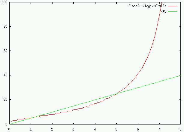
Although we do not encourage this, you can turn in your program up to 7 days late (until June 8th). In order to "help you" finish the assignment over the weekend before all your finals, we devised a logarithmic curve for docking points. Instead of the usual 5% per day, you will be docked floor(-1/log(x/8)*12) percent for every x days late. That way you are docked either the same or less than usual until sunday, but then you are docked quite a bit more afterwards.
Note, that the function is undefined for x = 0 (no such thing as log 0) because that is the day you should turn in the assignment for full credit. Furthermore, the function is undefined for x = 8 (division by zero) because by then it is too late to turn in any work. For your convenience, the following table will tell you the exact number of points you will be docked for each late day:
                             Day 1 (Wednesday)  5%
                             Day 2 (Thursday)   8%
                             Day 3 (Friday)    12%
                             Day 4 (Saturday)  17%
                             Day 5 (Sunday)    25%
                             Day 6 (Monday)    41%
                             Day 7 (Tuesday)   89%