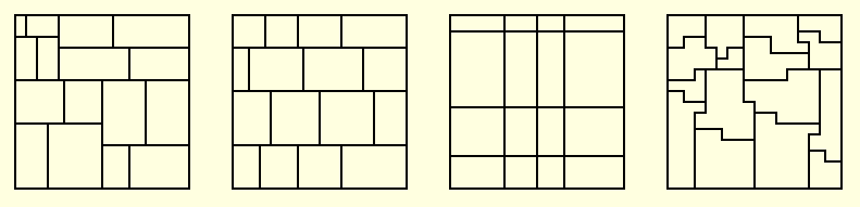
The Orthogonal Sectioning family of partitionings, from left to right: (a) ORB, (b) ORB-H, (c) rectilinear, and (d) ORB-MM.
Load sharing, which we discussed in Lecture 12, is a passive technique in that no attempt is made to actively respond to workload variations. An alternative is to actively measure workload variations and to partition the workloads non-uniformly so that each processor gets fair piece of the work. The pieces of work assigned to processors have different sizes according to the spatial density distribution of the work. In effect this is an off-line algorithm.
In general non-uniform partitioning will only work of we have a good idea of the workload distribution. If the distribution changes with time, then we may have to periodically repartition the work. In most physical problems, the solution changes gradually enough that the cost of repartitioning won't be too great. Non-uniform partitioning strategies are numerous, and we'll discuss one common approach: Orthogonal Recursive Bisection Orthogonal Recursive Bisection(ORB) (also known as Recursive Coordination Bisection (RCB)) is a useful non-uniform partitioning strategy. (M. J. Berger, S. H. Bokhari: "A Partitioning Strategy for Nonuniform Problems on Multiprocessors." IEEE Transactions on Computers 36(5): 570-580 (1987)).
It works by splitting the computation into to equal parts (of work, not space), and recursively splitting each part until done. ORB works when the number of processors is not a power of two, and it can be applied to multidimensional problems.
Consider the following loop:
  for (i = 1; i < N-1; i++)
	if (x[i] < 0)
	    y[i] = f1( x[i], x[i-1] );
	else
	    y[i] = f2( x[i], x[i-1] );
	end if
Assume that f1() takes twice as long to compute as f2( ). Now, if x[ ] changes very slowly, then we can build a workload density mapping giving the relative cost of updating each value of x[ ]. Let's assume that the mapping is as follows:
1 1 2 1 2 2 2 1 1 1 1 1 1 2 2 1We split the above array at the point where the sum of the elements on either side of the split is as equal as possible.
  1  1  2  1  2  2  2  1  1  1  1  1  1  2  2  1
		      ^
		      |
		   Cut here
If we are running on 4 processors, then we split again, once for each part
  1  1  2  1  2  2  2  1  1  1  1  1  1  2  2  1
	     ^	      ^                 ^
             |	      |		        |
	   Cut #2   Cut #1	     Cut #3
We now have 4 partitions with 5, 6, 6, and 5 units of work respectively.
ORB reduces the higher dimensional partitioning problem to a set of simpler 1-dimensional partitioning problems, successively partitioning along orthogonal coordinate directions. Generally the cutting direction is varied at each level of the recursion to avoid elongated partitions that could lead to poorly-balanced workloads.
The following figure shows some relatives relatives of ORB:
The Orthogonal Sectioning family of partitionings, from left to right:
(a) ORB,
(b) ORB-H,
(c) rectilinear, and (d) ORB-MM.
In some cases we may want to section a coordinate into more than two pieces. ORB-H or hierarchical ORB is a technique that employs multi-sectioning: it splits the problem into p > 2 strips and recurses on each strip. This technique is also referred to as multilevel ORB.
The principal disadvantage of the orthogonal sectioning algorithms is the geometric constraint that all cuts must be straight-edged. Hence, a cut in d dimensions introduces a workload imbalance that is carried by a d-1 dimensional hyper-plane. A way around the difficulty is to section the dividing hyper-plane, too; this strategy is called ORB-MM, or ORB-``Median of Medians.'' (Shown above.) However, ORB-MM generates highly irregular partitionings in three or more space dimensions which for all practical purposes are unstructured. Since unstructured partitionings do not have a compact representation, they require additional software bookkeeping to manage non-rectangular iteration spaces appearing in application software. In addition, distributed mapping tables must be maintained on message passing architectures, at the cost of additional communication overheads and a further increase in the application's complexity.
As we mentioned earlier, computations often exhibit temporal locality, whereby the solution changes gradually, for example, due to a time-step constraint. An incremental approach to orthogonal sectioning may effectively exploit temporal locality by computing work gradients across the partition boundaries and shifting the boundaries accordingly. However, complications arise when a boundary moves, since all other boundaries introduced later on in the recursion will be affected. In effect, we trade off temporal locality against spatial locality, and the trade-off may not be favorable. An approach which exploits temporal locality without the drawback of disrupting spatial locality is Nicol's rectilinear partitioning strategy. (Shown above.) This strategy avoids the difficulty of awkward workload adjustments by imposing a fixed connectivity on the partitionings. Partitionings are formed by the tensor product of strips taken across orthogonal coordinate directions. Load balance is improved by iteratively adjusting cuts independently along each problem dimension as necessary.
Inverse space-filling partitioning (ISP) is an alternative technique that shares the desirable fine-grained load balancing characteristic of ORB-MM but with simplified bookkeeping. ISP is fast--- it does not incur the heavy time penalties of optimization techniques---and is therefore appropriate for dynamic problems. ISP works by drawing a Hamiltonian path through the mesh and subdividing the resultant 1-d path. This path is also referred to as an Inverse Spacefilling curve, from which the method ``Inverse Spacefilling Partitioning'' takes its name. Because ISP partitionings are logically 1-dimensional, they are easier to manipulate than unstructured partitionings rendered by strategies such as ORB-MM. (If you are interested in learning more about these see Dynamic Partitioning of Non-Uniform Structured Workloads with Spacefilling Curves, by J. R. Pilkington and S. B. Baden. IEEE Trans. on Parallel and Distributed Systems , 7(3), March 1996, pp. 288-300.)
In addition to the above techniques there are also optimization methods. Typical approaches are based on simulated annealing, neural networks, and genetic algorithms. Approaches based on optimization are attractive because they balance workloads particularly well---they are fine-grained, mapping each point individually to a processor---and they also minimize communication. However, the benefits must be weighed against the cost: long and sometimes unpredictable running times. For this reason, optimization techniques are restricted to static problems. (A well known optimization approach is known as spectral graph decomposition. We'll talk about these in CSE 262.)
Software support for irregular decompositions is usually found in an application library. In addition to the decomposition utilities, we will also need some help in handling communication in message passing implementations. This is true because processors need to determine which neighbors they will communicate. Data will generally be non-contiguous, and must be packed into contiguous messages for transmission, and unpacked on the receiving side. One way of dealing with this is to use a library like KeLP.